Abstract
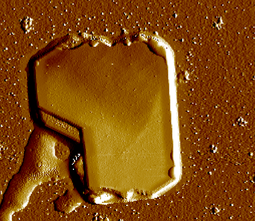
The Park Systems atomic force microscope was used to obtain images of Au particles, as well as a platinum Ditelluride (\(PtTe_{2}\)) flake. A height-height correlation function was implemented to analyze the topography of Au particles. The image of the \(PtTe_{2}\) flake was further analyzed in order to obtain any well-defined angles of the two-dimensional material flake. It has been determined from the height-height correlation function that the roughness (\(\sigma\)) or the average effective grain size to be 52.11 nm with an uncertainty of 1.235 nm. The coherence length, \(\xi\), was found to be 835.3 nm with an error of 0.37 nm. The Hurst(H) value is 0.9204. Starting from the top and going clockwise, the angles of the \(PeTe_{2}\) flake we could determine were 123, 96, 244, 159, and 124 degrees.
Introduction
Atomic Force Microscopy (AFM) is a third wave surface scanning method used to measure properties such as friction, electrical forces, capacitance, magnetic forces, conductivity, viscoelasticity, surface potential, and resistance (“Atomic Force Microscopy Nanoscience Instruments” n.d.) at nanometer scale. It uses the Van der Waals force to analyze material properties of nanomaterials. One of the advantages the AFM has over Scanning Electron Microscopy (SEM) is that it can measure non-conductive thin films. This gives us the ability to measure biological and soft matter materials. SEM utilizes a beam of electrons to detect the electromagnetic interactions of the sample. The information from these interactions is used to create an image of the sample. However, since there is no direct contact between the device and the sample, the resolution can be limited. In an AFM, we have a cantilever that can directly touch the sample when measuring materials in static mode. Although direct contact is not necessary and we can set the measurements to be done in dynamic mode where the cantilever is near but not touching the sample(Garcı́a and Pérez 2002). Due to the proximity between the cantilever and sample, all kinds of interatomic and intermolecular forces can be detected. Some of these include magnetic forces, electrostatic forces, mechanical contact forces, and Van der Waals forces. The Lennard Jones potential is used to model weak Van der Waals bonds (“Van Der Waals Force - an Overview ScienceDirect Topics” n.d.) in a material:
$$V(r) = 4\epsilon[( \frac{\sigma}{r})^{12} -( \frac{\sigma}{r})^{6} ]$$
We observe that this potential is a suitable model for short range interactions. This is a significant aspect of the system that AFM takes into account.
There are two different modes that the AFM can operate on. They are static mode and dynamic mode. In static mode, the cantilever comes into contact with the sample, whereas in dynamic mode, the cantilever is allowed to oscillate in order to obtain the attractive and repulsive forces. For the purposes of this lab, the static mode was employed in order to obtain images for our samples.
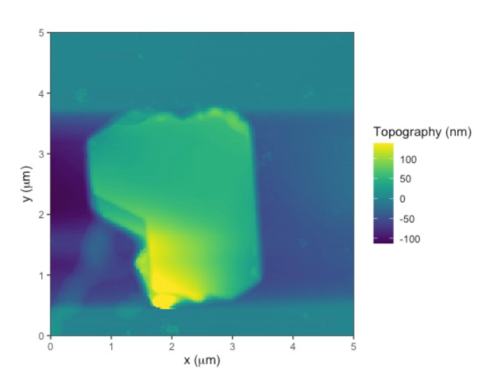
The samples analyzed in this lab were gold (Au) particles and platinum ditelluride \(PtTe_{2}\) flakes. In general, using AFM is a good way to determine the properties of materials. Using AFM imaging for Au particles allows us to obtain clear topographical characteristics of the material. This can shed light on the properties of these materials on the microscale. After AFM imaging is applied on the \(PtTe_{2}\) flake, we can determine the angles of two-dimensional material. Knowing properties about both of these materials can come in handy in the development of new technologies.
Experiment
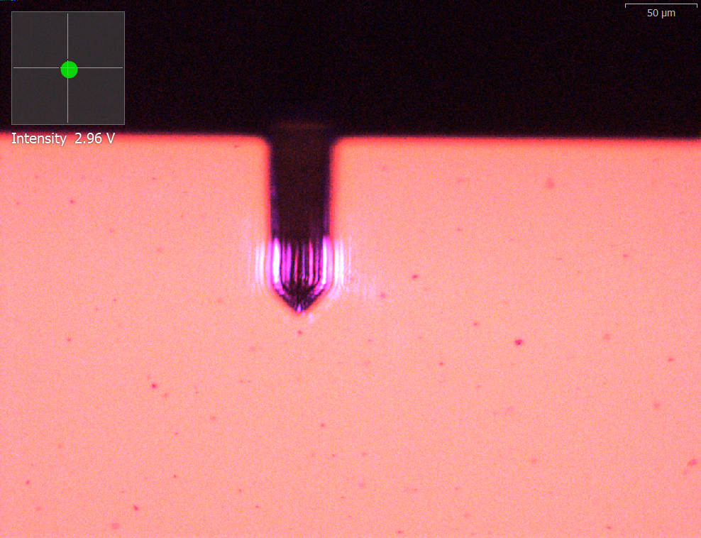
The first part of any experiment is to read the necessary manuals for all equipment that will be used. In the case of the Park AFM, we read sections of the Park AFM and the SmartScan software manuals. The first part is to turn on the computer, the control elements, and the activation table. With the instruments all on, the software was then turned on and given roughly 10 to 15 seconds for the program to reset. We ran a frequency sweep to ensure that all equipment was working within the acceptable range. After our scan we saw the Q factor at 9497 and the resolution frequency at 333.2kHz. We then logged that information as well as our names into the Park AFM logbook to leave a trail that all equipment is in working shape. We were now ready to work with the physical equipment. We need to make sure that the cantilever is both attached and intact. We unlocked the focal optics wheel by pushing a small lever back, turned the wheel until the cantilever was visible (noting it was visibly undamaged), then pulled the lever back gently until there was a slight resistance indicating the wheel was locked and can be let go of. The data is recorded by a quadrant photodiode (QPD) that receives the information via an infrared laser that is shone at an angle onto the cantilever and reflected back into the position sensing QPD. On the Smartscan software there is a position section that once clicked, has the values of the lateral, horizontal, and intensity values displaced. By moving the knobs on the XY stage, the beam was positioned on the cantilever, and the horizontal and lateral values were minimized with a vertical value of -0.3V and horizontal value of +0.14V. The intensity would rise and fall as the beam moved, but with minimal displacement, the intensity sum was a value of 2.97V which was close enough to the desired 3V value we were working towards. The next step is a visual quadrantrant check. The beam is shown in a square area depicted by a disk. If the beam is at the optimal spot, the disk is green, but if the beam needs more adjusting, the disk will appear as red.
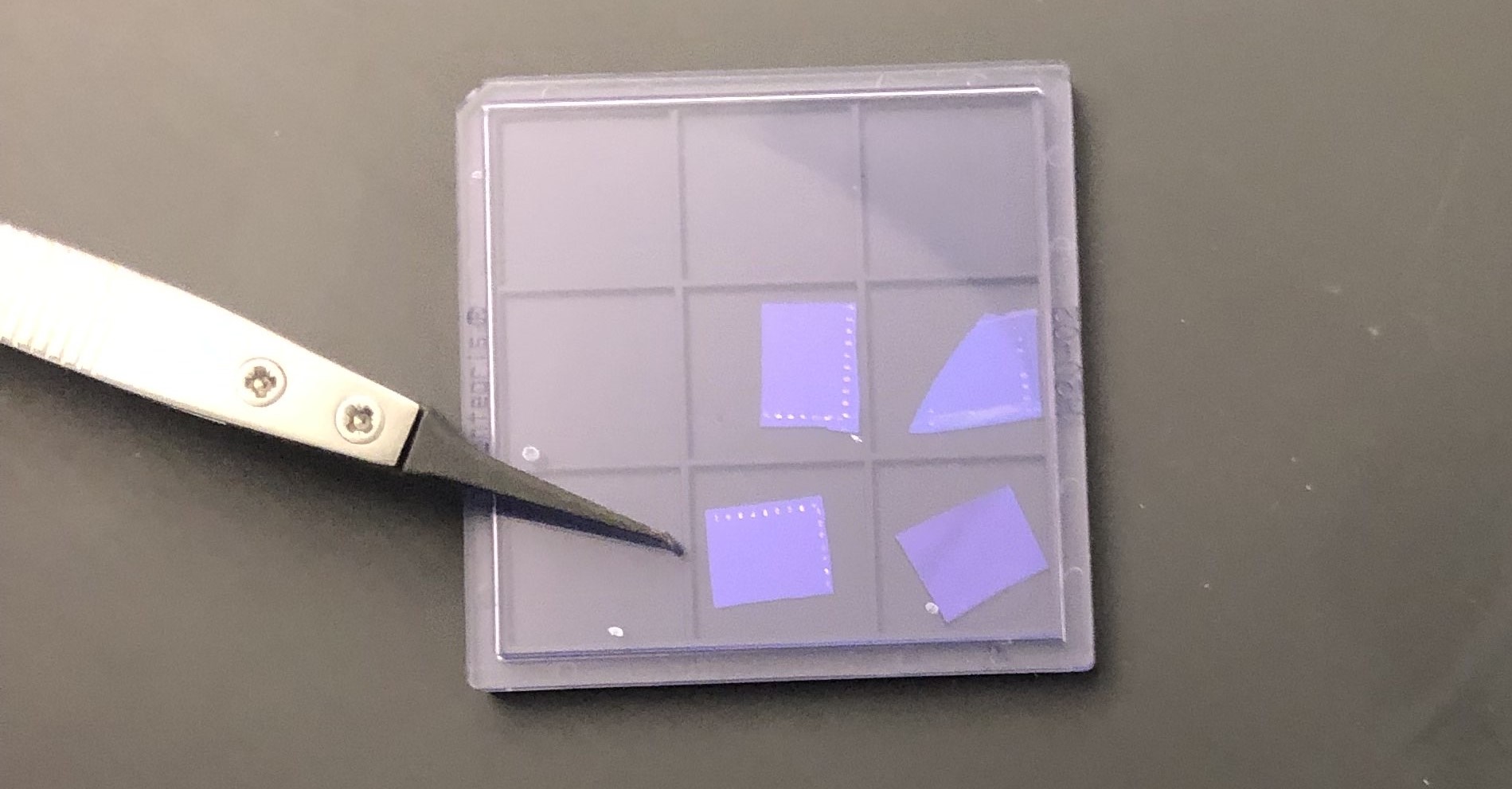
Once the beam is centered and green and the intensity close to 3V, we began to prep the sample. To keep a sanitary loading station, gloves were put on, placed a kimwipe on the table and pulled a pair of tweezers to handle the sample. To load the sample on the sample mount, we snipped a small piece of double sided tape,placed it on the mount, revealed the other side of the adhesive and lightly touched the adhesive a few times. This was to remove some adhesive to make the sample removal easier so no risk of damaging the adhesive. The sample was placed on the tape making sure that a corner is off the adhesive for a removal ledge. The stage and the mount are both magnetized, so when placing the mount on the stage, it was important to load the mounted sample by bringing it slowly from the side then raising it just enough to place on the magnet. This caution was exercised so the sample mounted stage didn’t hit the stage and damage the sample. Our first experiment was to examine a flake of gold. The specific sample used was T020200122Si16. As an optional step, we chose to readjust the focal optics so the camera could see the sample in focus rather than the cantilever, and saved the image.
With the sample loaded, we ran the image function on the Park AFM, and we had our first scan. We set the scan window to be 50μm by 50μm, the resolution to be 256 pixels and ran the Image function. We saved a snapshot of the topology the scan yielded of the sample under the file name 2024913_PHYS545_JCCBAB_AFM_T020200122Si16. The folder made to hold the data was named 2024913_PHYS545_JCCBAB_Au depicting the date, the class, the initials of the lab members, and the sample name for the file as well as element for the folder. The scan took place and the cantilever was automatically moved down to the surface of the sample. The scan revealed the surface as well as any debris. If any debris was detected, the best course of action would be to move the scan parameters to avoid this, which is exactly what we did as there was a small piece of debris detected under our initial sweep. We ran a few scans to optimize the parameters and saved all data.
With all the data collected, saved, properly named, and stored, we began the clean up procedure. The first part is to unlock the focal optics and turn the wheel to move the optic to the top, then relock. As with all types of AFM’s, taking care to not break the cantilever tip is paramount. There is an automatic lift button on the software we clicked and let the cantilever lift. Then the end button was clicked which lifted the cantilever up a substantial amount. Unfortunately, the end button does not always lift the cantilever up all the way, so the end button must be clicked up to 4 or 5 times to have the tip a safe distance raised. With the tip raised to a safe distance, the sample loaded mount was able to be carefully pulled to the side and down to remove just as carefully as it was initially placed. The sample loaded mount is to be placed on a clean Kimwipe, and the sample is to be removed from the mount using tweezers and placed back in its storage box. The double sided adhesive can be thrown away, and the mount placed back in the Park AFM toolbox. The software is then shut down, taking roughly 10 seconds or so. When the software is fully closed, the AFM controller, computer, and activation time are turned off. The sample is returned to where it belongs and the toolbox was placed back under the table on top of the computer. With everything shut down and put away, the last step of the clean up procedure is to sign the logbook with the state of the cantilever being intact.
Our next experiment was with a sample of Platinum Ditelluride. We turned on the computer, the activation table, and the AFM controller. The software was turned on and the frequency sweep was done. We chose one of four available options of Platinum Ditelluride samples to work with and prepped gathered the materials for mounting.
The values were logged into the log book with our names and the new date. The new sample we were using was put down as well. The sample was mounted with the double sided adhesive and carefully placed on the stage. The focal optics were moved into place to see the cantilever intact and the sample was prepped. We made a new folder 20240920_PHYS545_JCCBAB_SL20240916 for the new data from the day. We took a snapshot of the sample as seen by the camera and named the file 20240920_PHYS545_JCCBAB_SL20240916_Sample_Position. We ran the position function in the SmartScan software to position the cantilever on the sample, then ran the Image function. The scan of the first image was taken at 5μm by 5μm and was saved under the file name 20240920_PHYS545_JCCBAB_SL20240916_5um. Unfortunately there was no flake detected at this spot, and another scan was run at 20μm by 20μm with a lower resolution of 128 pixels to speed up scan time. With a flake detected, the scan parameters were adjusted back down to 5μm by 5μm around the flake and another scan was taken named 20240920_PHYS545_JCCBAB_SL20240916_5um_128x. Happier with these results, the resolution was increased back to 256 pixels and the data was saved under 20240920_PHYS545_JCCBAB_SL20240916_5um_256px.
With all data saved, the clean up procedure was begun. The focal optics were raised to the top, the cantilever was lifted 50μm at a time by pressing the lift button followed by the end button several times, and the sample was removed. The sample was carefully removed off of the sample mount and placed back into its proper storage container, the adhesive was thrown away, and the sample mount was put back in the AFM toolbox with the tweezers used to remove the sample. The software is shut down next, followed by turning off the activation table, AFM controller and the computer. With everything shut down, turned off, and put away, the log book is signed out with the status of the cantilever and the experiment is done.
Results and Analysis
We used the nanoAFM and ggplot2 packages on R to collect and plot the Park AFM data. The nanoAFM package to open the Park AFM data. Using a height-height correlation function we found the average effective grain size of Au particles and a single \(PtTe_2\) flake. The correlation function finds values of roughness (\(\sigma\)), coherence length (\(\xi\)), and the Hurst value (H) which is used to measure the persistance of an effective grain. We also measured the angles of defined edges of a \(PtTe_{2}\) projection using a protractor. The HHCF is defined as:
\(g(r) = \langle \left[ h(\vec{x}) - h(\vec{x} - \vec{r}) \right]^2\rangle\)
When r is the displacement vector. The height correlation fit we used in the data analysis was:
\(g(r) = 2 \sigma^2[ 1 - e^{-( \frac{r}{\xi})^{2/H}}]\)
\(\sigma\) is roughness, \(\xi\) is coherence length, and H is the Hursh value.
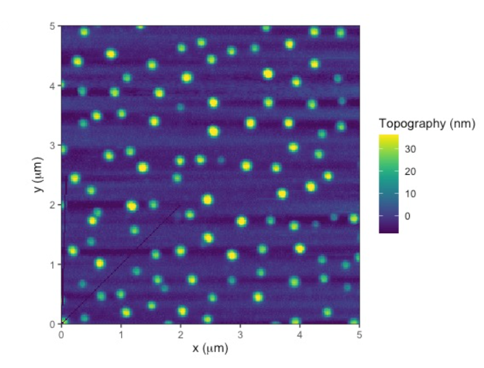
Using the nanoAfm package in R we found the height of the gold particles using the profile function. We saw that the gold particles have a roughly uniform shape and are not compact. The gold particle heights hovered around 20 to 30 nm. The difference in heights could be a result of deformation of gold particles after being transferred to the substrate or deformations of the Silicon substrate.
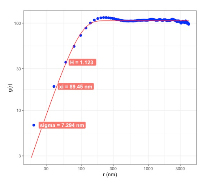
Using the nanoAFM package the HHCF found the roughness (\(\sigma\)) of the effective grain size to be 7.294 nm with an uncertainty of 0.009 nm which is on the order of pm. The coherence length, \(\xi\), to be 89.45 nm with an error of 1.93 nm. The H value is 1.123. These values could be because the surface isn’t homogeneous so H isn’t an accurate value for gauging roughness.
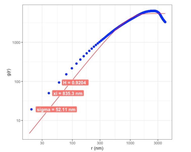
The HHCF found the roughness (\(\sigma\)) of the average effective grain to be 52.11 nm with an uncertainty of 1.235 nm. The \(\xi\) to be 835.3 nm with an error of 0.37 nm. The H value is 0.9204. This could be because the surface isn’t even because we are looking at one flake next to a flat surface so we can determine that the roughness value isn’t an accurate fit.
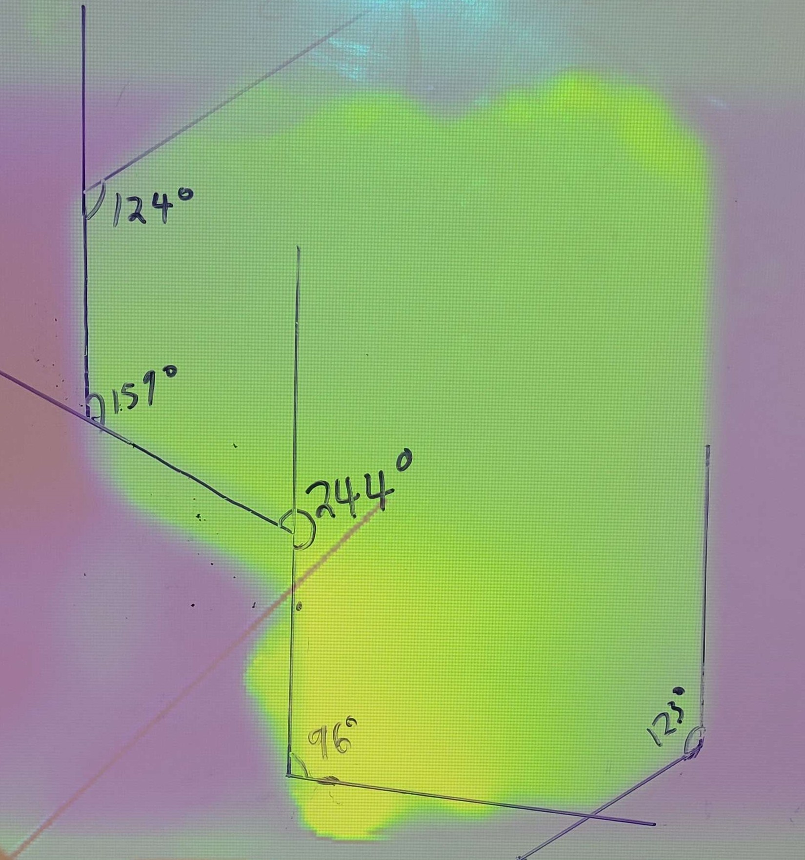
Rather than using software, the image was projected and a protractor was utilized to determine the well-defined angles of the two-dimensional flake. In our case, our uncertainty is about 1 degree, as that is what the smallest increment in the projector we used was. This is about what we’d expect from a two-dimensional material. Though not all of the sides of the flake have well-defined angles, we do expect at least some because platinum ditelluride is considered a two-dimensional molecule, thus when cutting up the lattice, these well-defined angles are expected to emerge.
Conclusion
AFM is a useful way to determine the properties of different materials on the microscale. This form of imaging has many advantages over other forms of microscopy, such as SEM because it has the ability to image samples that are non-conductive. The physical contact between the cantilever and the sample is very advantageous because it allows us to accurately reconstruct images from forces other than the electromagnetic forces. In this experiment, we were able to analyze the topography of the particles using the height-height correlation and the shape of the two-dimensional \(PtTe_{2}\) flake by measuring the angles. Obtaining accurate topographical representations of such materials at such a small scale provides insights for how it may be implemented among other materials. Knowledge about the properties of these materials can help us explore different possibilities for the fabrication of new technologies.
Acknowledgments
This project was assisted in part by Dr. Thomas Gredig and Filipe with their assistance safely using the PARK AFM. I would also like to thank the people who took the time to make the samples provided by Dr. Gredig that were used in our experiments.